Introduction:
The fine structure in x-ray has been known for over 40 years and can be considered as a unification of both x-ray diffraction and spectroscopy technique 1,2,3. Resonant elastic X-ray scattering (REXS) refers to a technique based on tuning the x-ray photon’s energy and measuring at the same time the intensity of a Bragg reflection. Near the absorption edge, the scattering power of the resonant atom is changed. This property provides thus a contrast between elements having close atomic number.
principles in few words:
The usual x-ray scattering from an atom consists of a Thompson or “free electron” contribution, characterized by the atomic form factor \(f_0\), as well as an resonant contribution characterized by the resonant form factors \(f^{\prime}+if^{\prime\prime}\).
\(f_0\) which is simply the Fourier transform of the electronic density can be well approximated using the Cromer-Mann4 equation : \(f_0(Q)=c+\sum_{i=1}^{4}a_i e^{(-b_i Q^2)}\) where \(Q=\frac{sin\theta}{\lambda}\). It is a bit more complicated for the resonant form factors because they are “material dependent” (see graph below). In the case of free atoms, the energy variation of both \(f^{\prime}\) and \(f^{\prime\prime}\) is given by the Sasaki tables5.
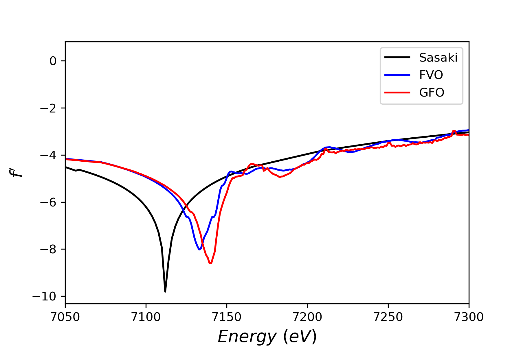
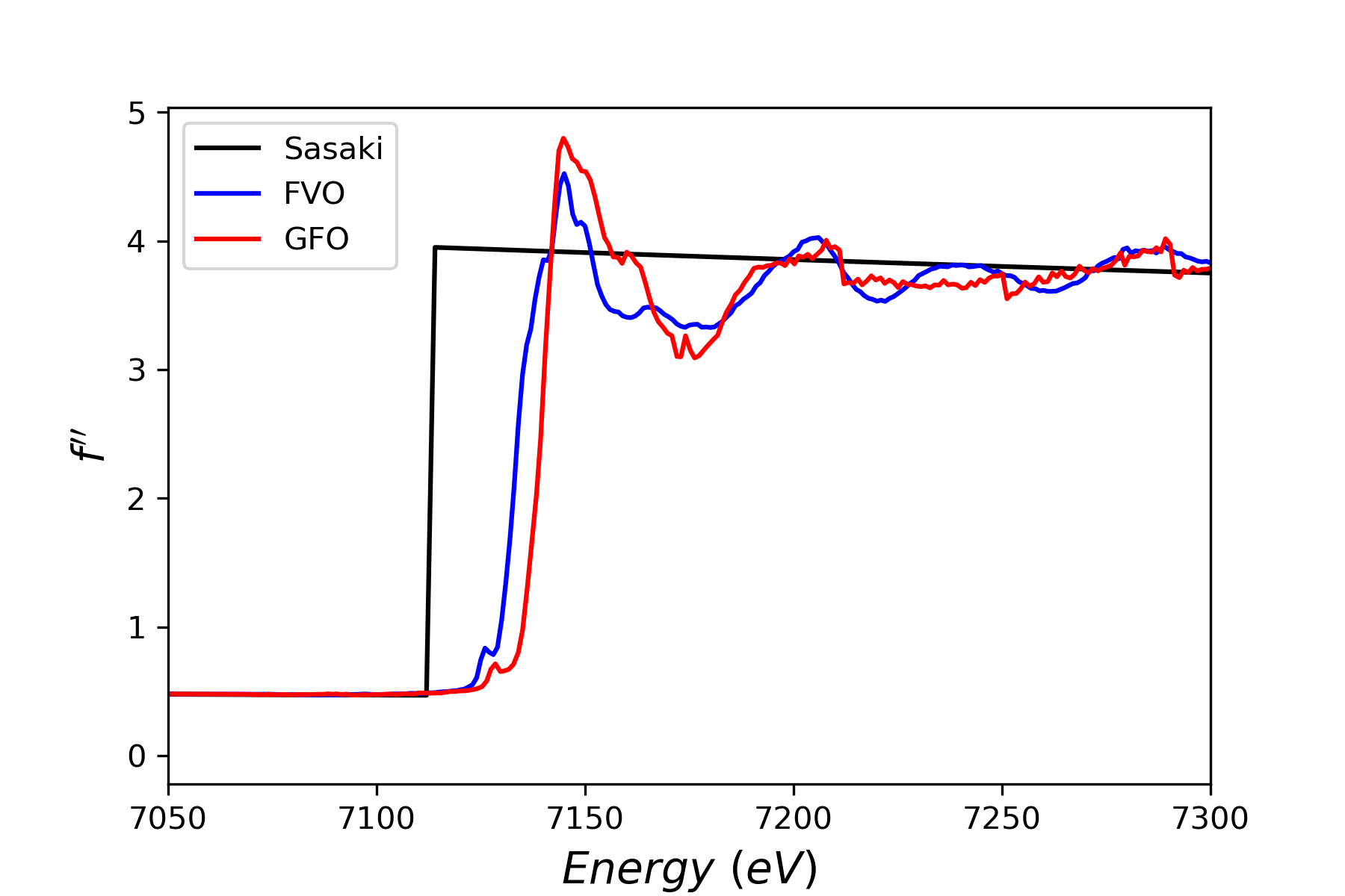
\(f^{\ \prime}\) (left) and \(f^{\ \prime\prime}\) (right) of free atoms (i.e. Sasaki values), \(FeV_2O_4 (=FVO)\) and \(Ga_{0.6}Fe_{1.4}O_3 (=GFO)\) compounds at the Fe edge
When the incoming photon’s energy, E, is near an atom’s atomic absorption edge,that photon can be absorbed by an electron (usually K or L shell) which is then expelled : this is the resonant behaviour which results in an abrupt change of both \(f^{\prime}\) and \(f^{\prime\prime}\). In that case, the structure factor changes significantly and it allows to probe e.g. crystallographic information of the resonant atom within the structure.
Classical analogy:
Let one electron moving around the nuclei. Since the electron is bounded, its displacement provides a harmonic restoring force and therefore a resonant frequency, \(\omega_r\).
When an incident electric field \(E_{in}=E_0e^{i\omega (t-r/c)}\)of x-ray beam drives the electron, the system can be classically described by a forced damped oscillator for which equation of motion is \(\frac{d^2x}{dt^2}+\beta\frac{dx}{dt}+\omega_r^2x=\frac{eE_0}{m}e^{-i\omega (t-r/c)}\) where x is the direction of the incident electric field \(E_0\).
the \(\beta\) parameter is proportional to the damping factor and \(\omega\) is the frequency of the incident wave. The solution of the differential equation is \(x(t)=\frac{eE_0}{m}\frac{e^{-i(\omega t-r/c)}}{\omega_r^2-\omega^2+i\beta\omega}\). It’s product by the charge of electron is an oscillating dipole moment for which the radiation intensity is proportionnal to its acceleration. The ratio of the radiated to incident electric fields is given by : \(\frac{E_{rad}}{E_{in}} \propto \frac{\omega^2}{\omega^2-\omega_r^2+i\beta \omega} \frac{e^{i\omega r/c}}{r} \).
The atomic form factor (labelled f) is defined as the amplitude of the outgoing spherical wave of previous result. It leads to \(f = \frac{\omega^2}{\omega^2-\omega_r^2+i\beta \omega}\).
Let’s change the equation in order to show the Thomson term (Z = 1 here):
\(f = 1+\overbrace{\frac{\omega_r^2-i\omega\beta}{\omega^2-\omega_r^2+i\beta\omega}}^{f^\prime + if^{\prime\prime}}
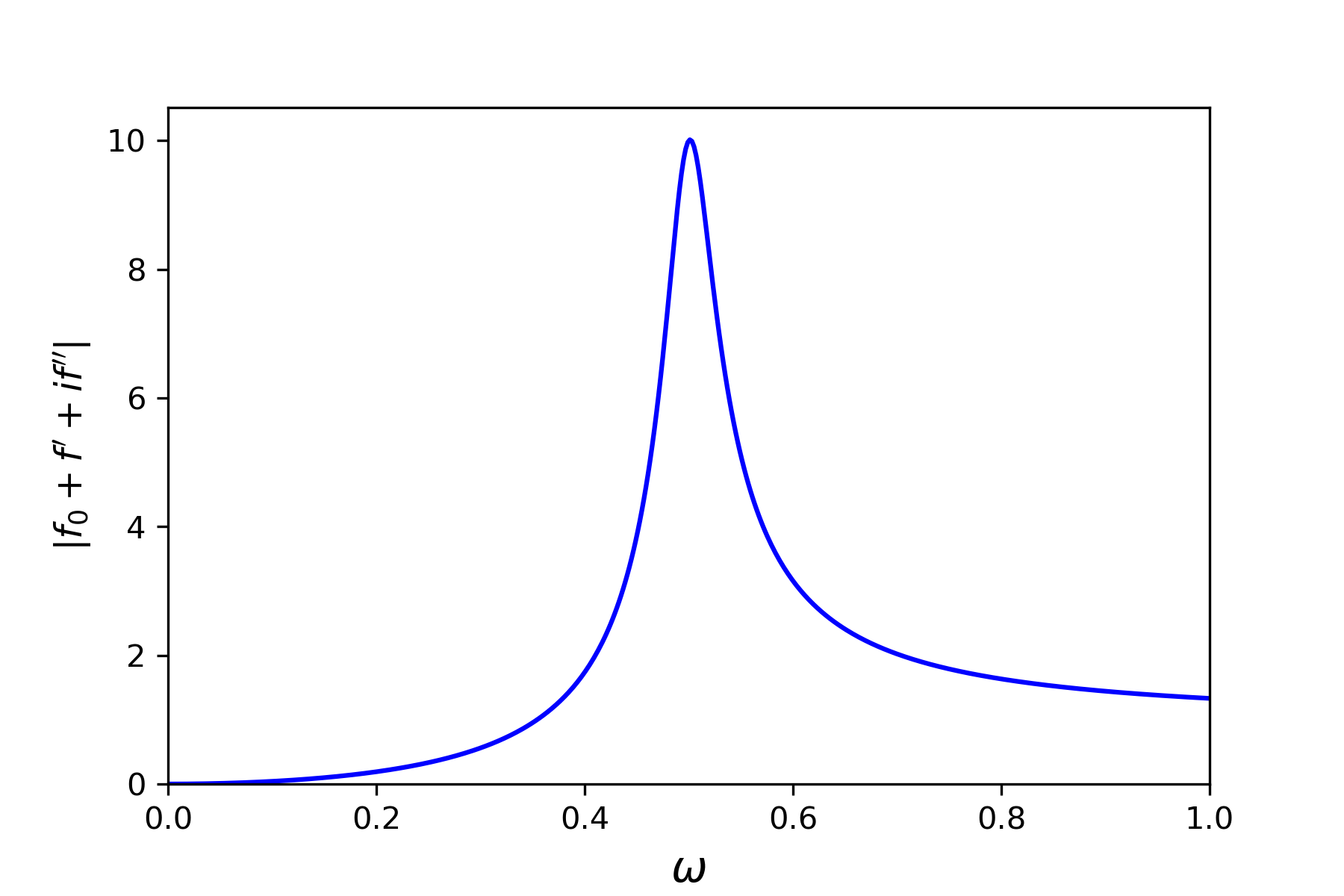
\). One obtains finally : \(f=f_0+f^{\prime}(\omega)+if^{\prime\prime}(\omega) = 1 + \underbrace{\frac{\omega_r^2(\omega-\omega_r^2)-(\omega\beta)^2}{(\omega^2-\omega_r^2)^2+(\omega\beta)^2}}_{f^{\prime}} \underbrace{-i\frac{\beta\omega^3}{(\omega^2-\omega_r^2)^2+(\omega\beta)^2}}_{f^{\prime\prime}}\). The curves associated to the different terms are represented below.
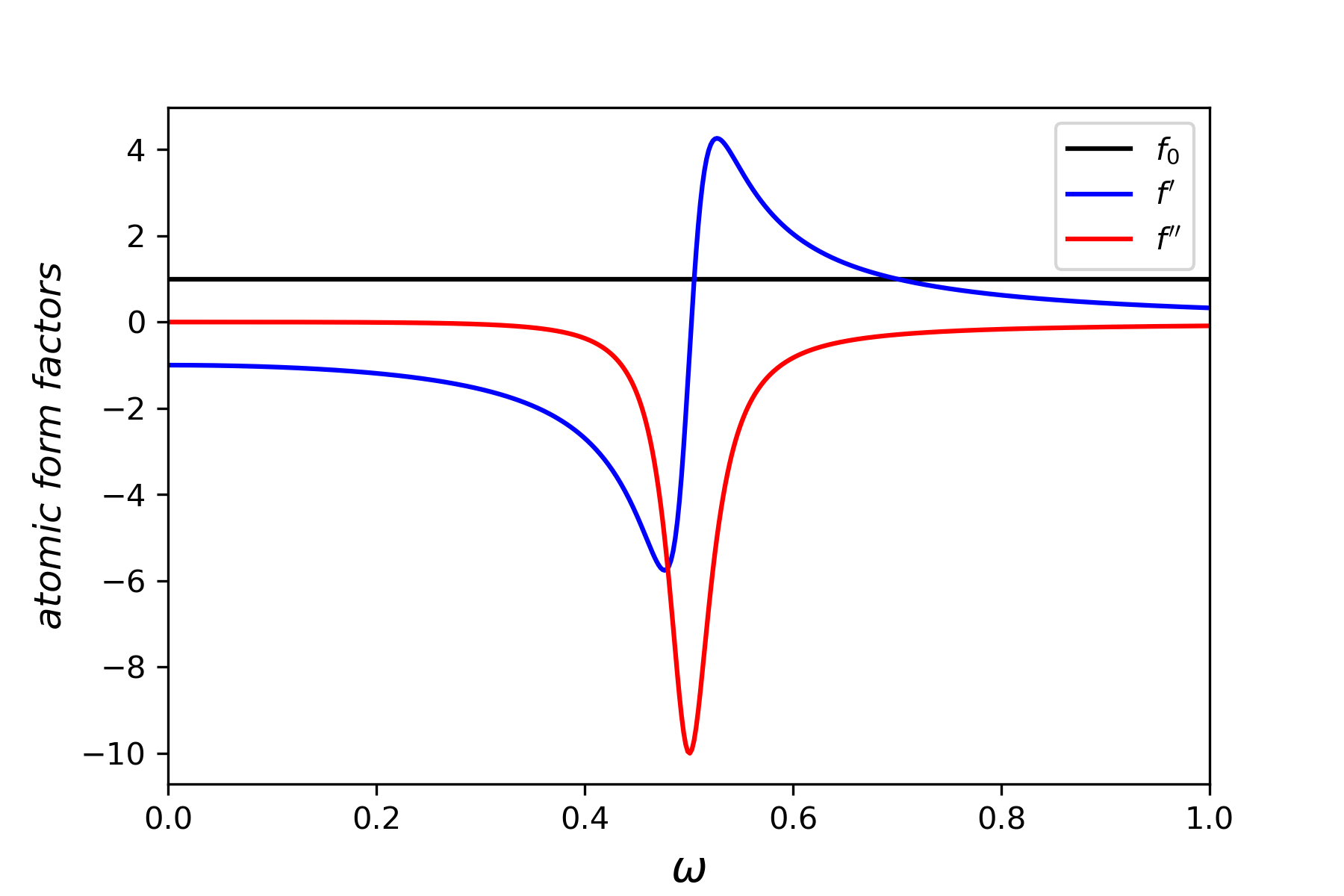
Computed atomic form factors from classical equation. \(\omega_r\) and \(\beta\) have been arbitrary choosen equal to 0.5 and 0.05, respectively
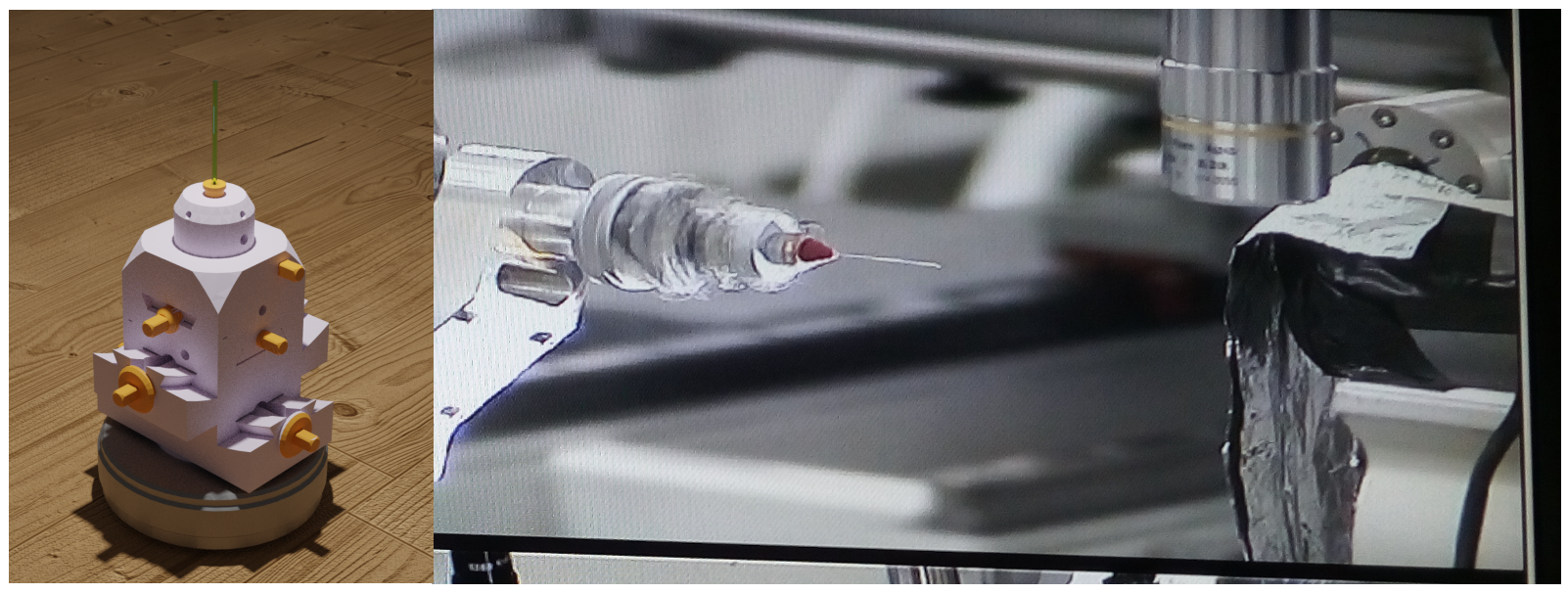
Experimental setup:
X-ray anomalous diffraction experiments can be performed using tunable energy of the synchrotron near the absorption edge. Our team performed acquisitions at both D2AM and Diffabs beamlines at ESRF and Soleil, respectively.
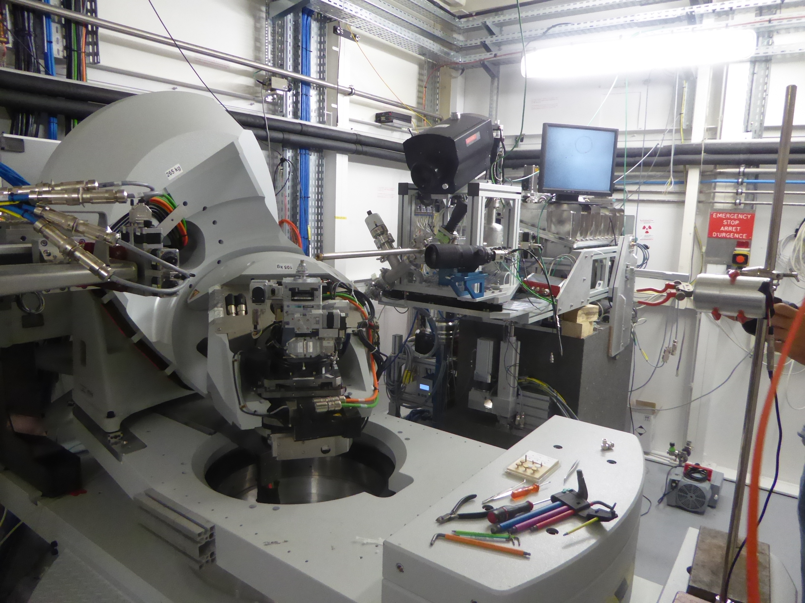
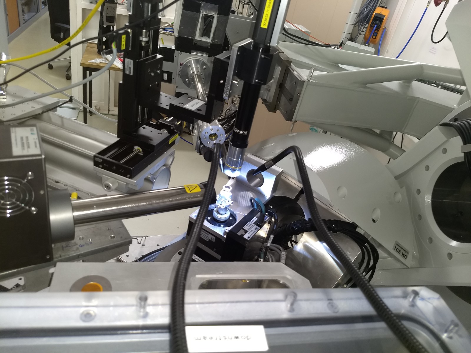
d2am (left) and diffabs (right) beamlines
Acquisition:
• Thin film sample
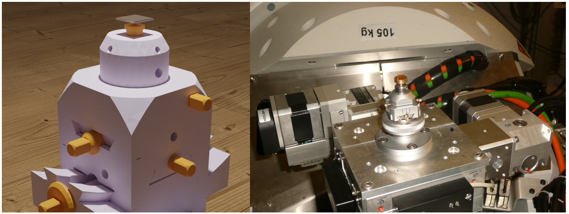
Sample is mounted on a goniometer head on a diffractometer equipped with various photodiode detectors, allowing e.g. recording of intensity of the incident beam \(I_0\) or the fluorescence of the samples. For each sample, the rotation matrix is preliminarily determined with the help of different in-plane and out-of-plane reflections.
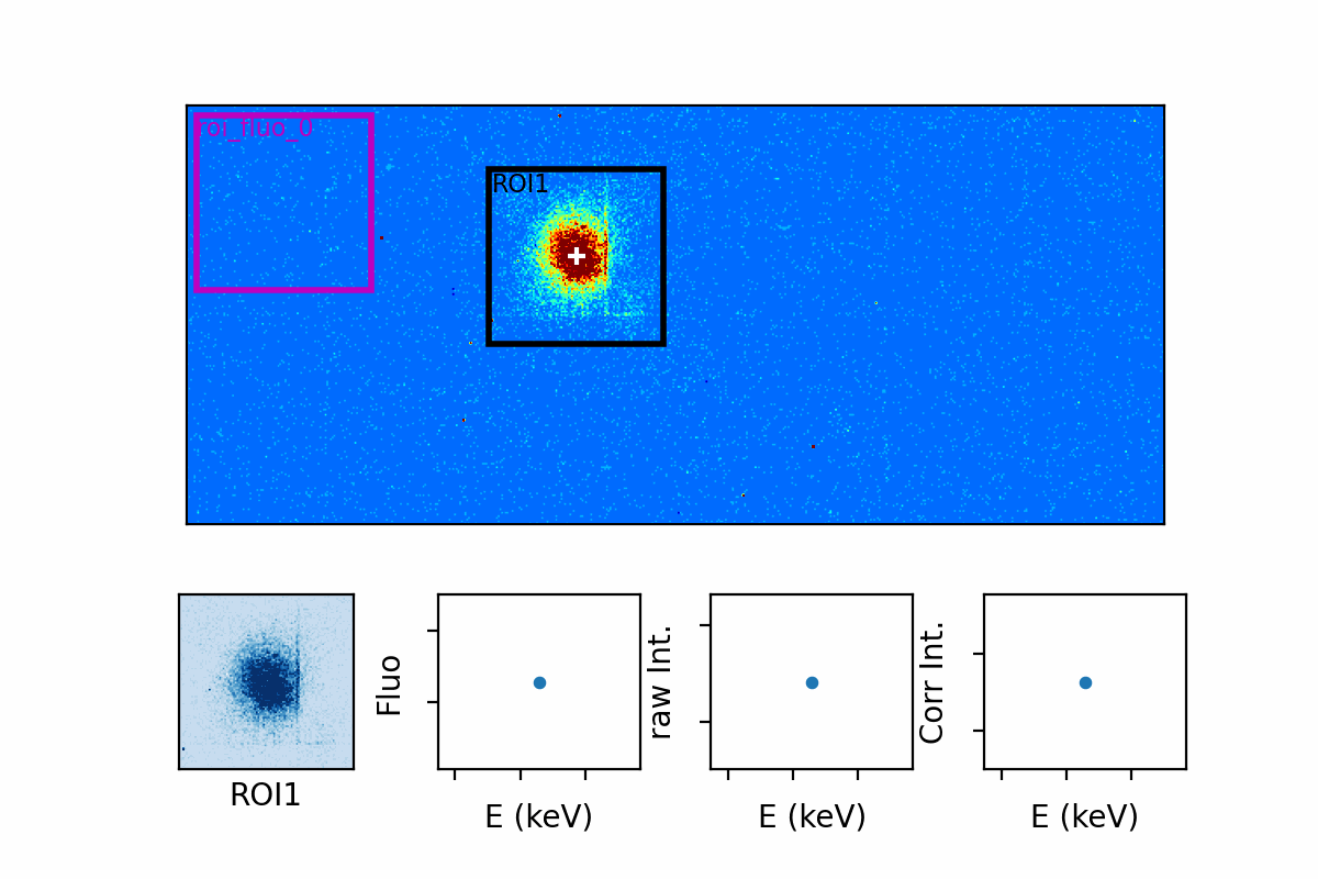
evolution of the 204 node of \(Ga_{0.6}Fe_{1.4}O_3\) thin films at Fe edge. Bottom graphs are (from left to right) : 1) the region of interest (ROI) centered at the diffracted node, 2) the evolution of the fluorescence with energy, 3) evolution of raw intensity with energy and, 4) evolution of corrected intensity with energy. nb : in this configuration, the detector was fixed explaining the motion of the node with energy
• Powder sample
The characterization of powders is much more delicate to implement because of the absorption of the signal by the solid material. However it’s possible to perform measurement if the sample is finely ground and placed in a capillary with a maximum diameter of 0.3 mm.

evolution of the 333 ring (located in the black ROI) of \(FeV_2O_4\) powder at Fe edge. Bottom graphs are (from left to right) : 1) the evolution of the fluorescence with energy, 2) evolution of raw intensity with energy and, 3) evolution of corrected intensity with energy. nb : in this configuration, the apparent immobility of the node is explained by the fact that the detector was moving at the same time so that the recording was made on the same area of pixels.
Exploitation of experimental data:
softwares:
We use 2 codes in order to fit the experimental data:
• FitREXS: developped at IPCMS, it allows to perform simulation and/or simultaneously refinement of anomalous x-ray spectra. FitREXS uses experimental fluorescence data to extract the anomal factors.
• FDMNES :
developped at the Neel Institut, it’s a friendly ab initio code which allow to simulate X-ray absorption and emission spectroscopies as well as resonant x-ray scattering and x-ray Raman spectroscopies, among other techniques.
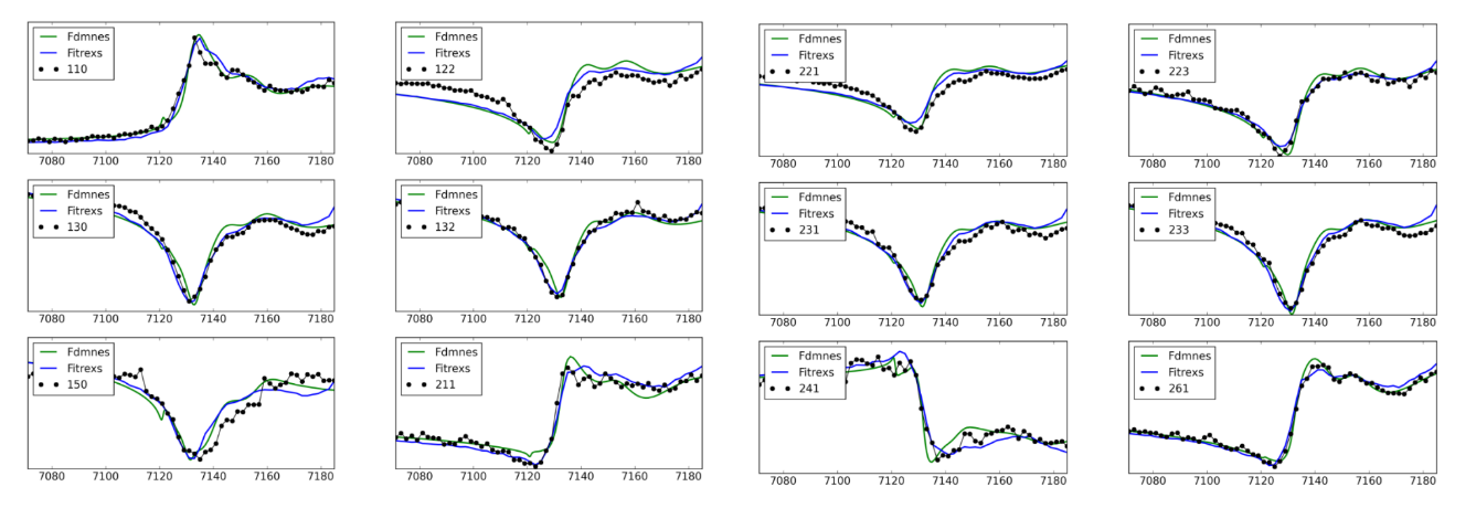
Experimental data and refinement using Fdmnes (green) and FitREXS (blue) of \(Ga_{0.6}Fe_{1.4}O_3\) thin film at the Fe edge [6]
references:
[1] Y. Cauchois, C. R. Acad. Sci. 242, 100 (1956).
[2] C.J.S. edited by G. Materlik, Resonant Anomalous X-Ray Scattering: Theory and Applications (North-Holland, Amsterdam New York, 1994).
[3] S Grenier and Y Joly 2014, Basics of Resonant Elastic X-ray Scattering theory ,J. Phys.: Conf. Ser.519 012001
[4] Cromer, D. T. & Liberman, D. (1970). J. Chem. Phys. 53, 1891.
[5] Sasaki, S. (1989). Report KEK 88-14. National Laboratory for High
Energy Physics, Japan.
[6] C. Lefevre, A. Thomasson, F. Roulland, V. Favre-Nicolin, Y. Joly, Y. Wakabayashi, G. Versini, S. Barre, C. Leuvrey, A. Demchenko, N. Boudet, and N. Viart, Determination of the Cationic Distribution in Oxidic Thin Films by Resonant X-Ray Diffraction: The Magnetoelectric Compound \(Ga_{2− x}Fe_xO_3\), J. Appl. Crystallogr. 49, 4 (2016)